Combine multiple ggplot objects into a single layout

The multiplot function arranges multiple ggplot2 objects into a single plotting layout with a specified number of columns.

Usage

multiplot(..., cols = 1)

Arguments

...

One or more ggplot2 objects.

cols

Integer specifying the number of columns in the layout.

Value

A grid object displaying multiple plots arranged in the specified layout.

Details

Multiple ggplot2 objects can be provided either as separate arguments via .... The function uses the grid package to control the layout.

Author

Pedro J. (adapted from https://gist.github.com/pedroj/ffe89c67282f82c1813d)

Examples

# Example using output from TTEST_DDCt
data1 <- read.csv(system.file("extdata", "data_1factor_one_ref.csv", package = "rtpcr"))
a <- TTEST_DDCt(
  data1,
  numberOfrefGenes = 1,
  plotType = "log2FC")
#> *** 3 target(s) using 1 reference gene(s) was analysed!
#> *** The control level was used as calibrator.
p1 <- a$plot

# Example using output from ANOVA_DCt
data2 <- read.csv(system.file("extdata", "data_1factor.csv", package = "rtpcr"))
out2 <- ANOVA_DCt(
  data2,
  numOfFactors = 1,
  numberOfrefGenes = 1,
  block = NULL)
#> NULL
#> 
#> Relative expression (DCt method)
#>   SA     RE  log2FC    LCL    UCL     se Lower.se.RE Upper.se.RE
#> 1 L3 0.9885 -0.0167 1.5318 0.6379 0.0841      0.9325      1.0479
#> 2 L2 0.6271 -0.6733 0.9717 0.4047 0.4388      0.4626      0.8500
#> 3 L1 0.2852 -1.8100 0.4419 0.1840 0.0208      0.2811      0.2893
#>   Lower.se.log2FC Upper.se.log2FC sig
#> 1         -0.0177         -0.0157   a
#> 2         -0.9127         -0.4968   a
#> 3         -1.8363         -1.7841   b
#> 
#> Combined Expression Table (all genes)
#>   gene SA     RE  log2FC    LCL    UCL     se Lower.se.RE Upper.se.RE
#> 1   PO L3 0.9885 -0.0167 1.5318 0.6379 0.0841      0.9325      1.0479
#> 2   PO L2 0.6271 -0.6733 0.9717 0.4047 0.4388      0.4626      0.8500
#> 3   PO L1 0.2852 -1.8100 0.4419 0.1840 0.0208      0.2811      0.2893
#>   Lower.se.log2FC Upper.se.log2FC sig
#> 1         -0.0177         -0.0157   a
#> 2         -0.9127         -0.4968   a
#> 3         -1.8363         -1.7841   b
  
df <- out2$combinedResults

p2 <- plotFactor(
  df,
  x_col = "SA",
  y_col = "RE",
  Lower.se_col = "Lower.se.RE",
  Upper.se_col = "Upper.se.RE",
  letters_col = "sig",
  letters_d = 0.1,
  col_width = 0.7,
  err_width = 0.15,
  fill_colors = "skyblue",
  alpha = 1,
  base_size = 16)

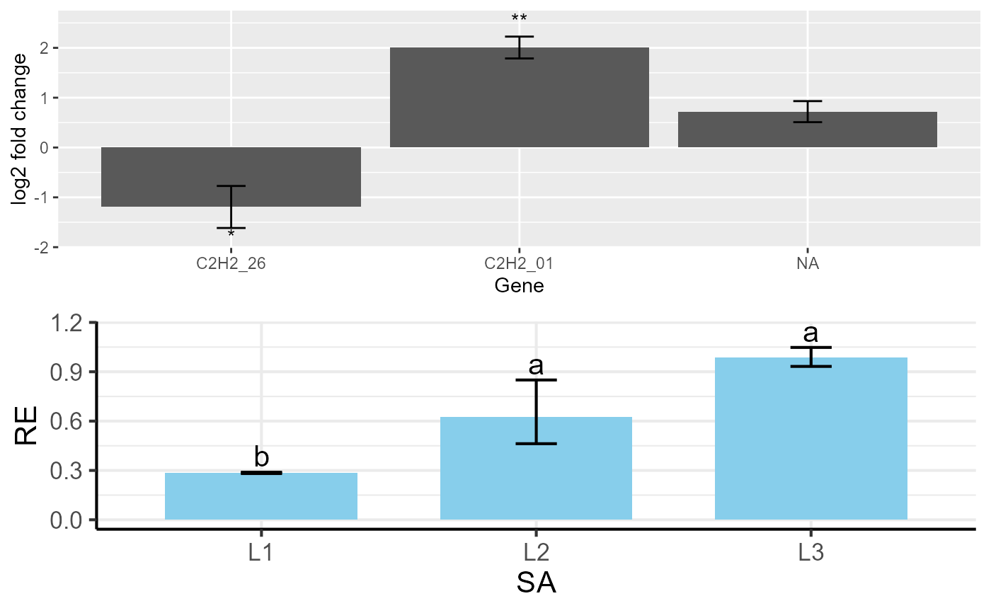
# Combine plots into a single layout
multiplot(p1, p2, cols = 2)


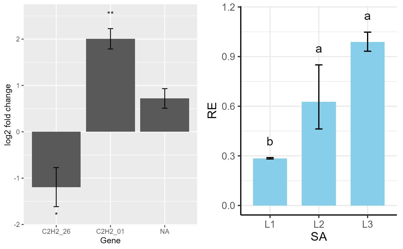multiplot(p1, p2, cols = 1)