Bar plot of gene(s) expression for 1-, 2-, or 3-factor experiments
Source:R/plotFactor.R
plotFactor.RdCreates a bar plot of relative gene expression (fold change) values from 1-, 2-, or 3-factor experiments, including error bars and statistical significance annotations.
Usage
plotFactor(
  data,
  x_col,
  y_col,
  Lower.se_col,
  Upper.se_col,
  group_col = NULL,
  facet_col = NULL,
  letters_col = NULL,
  letters_d = 0.2,
  col_width = 0.8,
  err_width = 0.15,
  dodge_width = 0.8,
  fill_colors = NULL,
  color = NA,
  alpha = 1,
  base_size = 12,
  legend_position = "right",
  removeCalibratorCols = FALSE,
  removeCalibratorText = FALSE,
  ...
)
Arguments
- data
Data frame containing expression results
- x_col
Character. Column name for x-axis
- y_col
Character. Column name for bar height
- Lower.se_col
Character. Column name for lower SE
- Upper.se_col
Character. Column name for upper SE
- group_col
Character. Column name for grouping bars (optional)
- facet_col
Character. Column name for faceting (optional)
- letters_col
Character. Column name for significance letters (optional)
- letters_d
Numeric. Vertical offset for letters (default
0.2)- col_width
Numeric. Width of bars (default
0.8)- err_width
Numeric. Width of error bars (default
0.15)- dodge_width
Numeric. Width of dodge for grouped bars (default
0.8)- fill_colors
Optional vector of fill colors to change the default colors
- color
Optional color for the bar outline
- alpha
Numeric. Transparency of bars (default
1)- base_size
Numeric. Base font size for theme (default
12)- legend_position
Character or numeric vector. Legend position (default
right)- removeCalibratorCols
= NULL or remove Calibrator Cols
- removeCalibratorText
= NULL or remove Calibrator text
- ...
Additional ggplot2 layer arguments
Examples
data <- read.csv(system.file("extdata", "data_2factorBlock3ref.csv", package = "rtpcr"))
res <- ANOVA_DDCt(x = data,
numOfFactors = 2,
numberOfrefGenes = 3,
block = "block",
specs = "Concentration",
p.adj = "none")
#>
#> Relative Expression
#> gene contrast ddCt RE LCL UCL log2FC se Lower.se.RE
#> 1 PO L1 0.00000 1.00000 0.00000 0.00000 0.00000 0.09187 0.93830
#> 2 PO L2 vs L1 -0.94610 1.92666 1.35851 2.73242 0.94610 0.13465 1.75497
#> 3 PO L3 vs L1 -2.19198 4.56931 3.30647 6.31447 2.19198 0.18224 4.02710
#> 4 NLM L1 0.00000 1.00000 0.00000 0.00000 0.00000 0.09017 0.93941
#> 5 NLM L2 vs L1 0.86568 0.54879 0.42187 0.71389 -0.86568 0.06252 0.52552
#> 6 NLM L3 vs L1 -0.51619 1.43017 1.08699 1.88170 0.51619 0.18103 1.26152
#> Upper.se.RE Lower.se.log2FC Upper.se.log2FC p.value sig
#> 1 1.06575 -0.09187 0.09187 1.00000
#> 2 2.11515 0.81145 1.08076 0.00116 **
#> 3 5.18453 2.00974 2.37421 0.00000 ***
#> 4 1.06450 -0.09017 0.09017 1.00000
#> 5 0.57309 -0.92819 -0.80316 0.00018 ***
#> 6 1.62137 0.33516 0.69722 0.01382 *
#>
#> The L1 level was used as calibrator.
#> Note: Using default model for statistical analysis: wDCt ~ block + Concentration * Type
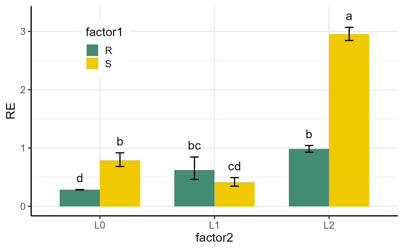
df <- res$relativeExpression
p1 <- plotFactor(
data = df,
x_col = "contrast",
y_col = "RE",
group_col = "gene",
facet_col = "gene",
Lower.se_col = "Lower.se.RE",
Upper.se_col = "Upper.se.RE",
letters_col = "sig",
letters_d = 0.2,
alpha = 1,
col_width = 0.7,
dodge_width = 0.7,
base_size = 14,
legend_position = "none")
p1
 data2 <- read.csv(system.file("extdata", "data_3factor.csv", package = "rtpcr"))
#Perform analysis first
res <- ANOVA_DCt(
data2,
numOfFactors = 3,
numberOfrefGenes = 1,
block = NULL)
#>
#> Relative Expression
#>
#> gene Type Conc SA dCt RE log2FC LCL UCL se
#> 1 PO R L A1 1.81000 0.28519 -1.81000 0.18241 0.44589 0.02082
#> 2 PO S L A1 0.33000 0.79554 -0.33000 0.50883 1.24380 0.21284
#> 3 PO R M A1 0.67333 0.62706 -0.67333 0.40107 0.98039 0.43880
#> 4 PO S M A1 1.27000 0.41466 -1.27000 0.26522 0.64831 0.25403
#> 5 PO R H A1 0.01667 0.98851 -0.01667 0.63225 1.54552 0.08413
#> 6 PO S H A1 -1.57000 2.96905 1.57000 1.89900 4.64204 0.05508
#> 7 PO R L A2 3.96333 0.06411 -3.96333 0.04100 0.10023 0.82277
#> 8 PO S L A2 -0.61667 1.53333 0.61667 0.98072 2.39732 0.08647
#> 9 PO R M A2 1.66667 0.31498 -1.66667 0.20146 0.49246 0.28898
#> 10 PO S M A2 0.33000 0.79554 -0.33000 0.50883 1.24380 0.25710
#> 11 PO R H A2 1.20333 0.43427 -1.20333 0.27776 0.67897 0.08373
#> 12 PO S H A2 -2.37667 5.19335 2.37667 3.32167 8.11969 0.13094
#> Lower.se.RE Upper.se.RE Lower.se.log2FC Upper.se.log2FC sig
#> 1 0.28111 0.28934 -1.83082 -1.78918 f
#> 2 0.68642 0.92200 -0.54284 -0.11716 cd
#> 3 0.46261 0.84996 -1.11213 -0.23453 cde
#> 4 0.34771 0.49450 -1.52403 -1.01597 ef
#> 5 0.93252 1.04787 -0.10080 0.06746 bc
#> 6 2.85784 3.08458 1.51492 1.62508 a
#> 7 0.03624 0.11340 -4.78610 -3.14057 g
#> 8 1.44412 1.62805 0.53019 0.70314 b
#> 9 0.25780 0.38484 -1.95565 -1.37768 f
#> 10 0.66568 0.95072 -0.58710 -0.07290 cd
#> 11 0.40978 0.46022 -1.28707 -1.11960 def
#> 12 4.74277 5.68675 2.24573 2.50760 a
#>
#> Note: Using default model for statistical analysis: wDCt ~ Type * Conc * SA
df <- res$relativeExpression
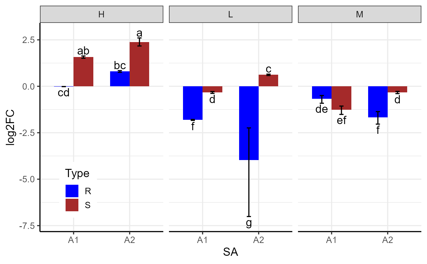
# Generate three-factor bar plot
p <- plotFactor(
df,
x_col = "SA",
y_col = "log2FC",
group_col = "Type",
facet_col = "Conc",
Lower.se_col = "Lower.se.log2FC",
Upper.se_col = "Upper.se.log2FC",
letters_col = "sig",
letters_d = 0.3,
col_width = 0.7,
dodge_width = 0.7,
#fill_colors = c("blue", "brown"),
color = "black",
base_size = 14,
alpha = 1,
legend_position = c(0.1, 0.2))
p
data2 <- read.csv(system.file("extdata", "data_3factor.csv", package = "rtpcr"))
#Perform analysis first
res <- ANOVA_DCt(
data2,
numOfFactors = 3,
numberOfrefGenes = 1,
block = NULL)
#>
#> Relative Expression
#>
#> gene Type Conc SA dCt RE log2FC LCL UCL se
#> 1 PO R L A1 1.81000 0.28519 -1.81000 0.18241 0.44589 0.02082
#> 2 PO S L A1 0.33000 0.79554 -0.33000 0.50883 1.24380 0.21284
#> 3 PO R M A1 0.67333 0.62706 -0.67333 0.40107 0.98039 0.43880
#> 4 PO S M A1 1.27000 0.41466 -1.27000 0.26522 0.64831 0.25403
#> 5 PO R H A1 0.01667 0.98851 -0.01667 0.63225 1.54552 0.08413
#> 6 PO S H A1 -1.57000 2.96905 1.57000 1.89900 4.64204 0.05508
#> 7 PO R L A2 3.96333 0.06411 -3.96333 0.04100 0.10023 0.82277
#> 8 PO S L A2 -0.61667 1.53333 0.61667 0.98072 2.39732 0.08647
#> 9 PO R M A2 1.66667 0.31498 -1.66667 0.20146 0.49246 0.28898
#> 10 PO S M A2 0.33000 0.79554 -0.33000 0.50883 1.24380 0.25710
#> 11 PO R H A2 1.20333 0.43427 -1.20333 0.27776 0.67897 0.08373
#> 12 PO S H A2 -2.37667 5.19335 2.37667 3.32167 8.11969 0.13094
#> Lower.se.RE Upper.se.RE Lower.se.log2FC Upper.se.log2FC sig
#> 1 0.28111 0.28934 -1.83082 -1.78918 f
#> 2 0.68642 0.92200 -0.54284 -0.11716 cd
#> 3 0.46261 0.84996 -1.11213 -0.23453 cde
#> 4 0.34771 0.49450 -1.52403 -1.01597 ef
#> 5 0.93252 1.04787 -0.10080 0.06746 bc
#> 6 2.85784 3.08458 1.51492 1.62508 a
#> 7 0.03624 0.11340 -4.78610 -3.14057 g
#> 8 1.44412 1.62805 0.53019 0.70314 b
#> 9 0.25780 0.38484 -1.95565 -1.37768 f
#> 10 0.66568 0.95072 -0.58710 -0.07290 cd
#> 11 0.40978 0.46022 -1.28707 -1.11960 def
#> 12 4.74277 5.68675 2.24573 2.50760 a
#>
#> Note: Using default model for statistical analysis: wDCt ~ Type * Conc * SA
df <- res$relativeExpression
# Generate three-factor bar plot
p <- plotFactor(
df,
x_col = "SA",
y_col = "log2FC",
group_col = "Type",
facet_col = "Conc",
Lower.se_col = "Lower.se.log2FC",
Upper.se_col = "Upper.se.log2FC",
letters_col = "sig",
letters_d = 0.3,
col_width = 0.7,
dodge_width = 0.7,
#fill_colors = c("blue", "brown"),
color = "black",
base_size = 14,
alpha = 1,
legend_position = c(0.1, 0.2))
p