Manual • rtpcr

Overview

Tools for analysis of RT-qPCR gene expression data using $\Delta Ct$ and $\Delta\Delta Ct$ methods, including t-tests, ANOVA, ANCOVA, repeated-measures models, and publication-ready visualizations. The package implements a general calculation method described by Ganger et al. (2017) and Taylor et al. (2019), covering both the Livak and Pfaffl methods. See the calculation method for details.

Functions

The rtpcr package gets efficiency (E) the Ct values of genes and performs different analyses using the following functions.

Function	Description
`ANOVA_DCt`	$\Delta Ct$ ANOVA analysis
`ANOVA_DDCt`	$\Delta\Delta Ct$ ANOVA analysis
`REPEATED_DDCt`	$\Delta\Delta Ct$ ANOVA analysis for repeated-measures data
`TTEST_DDCt`	$\Delta\Delta Ct$ method t-test analysis
`plotFactor`	Bar plot of gene expression for one-, two- or three-factor experiments
`Means_DDCt`	Pairwise comparison of RE values for any user-specified effect
`efficiency`	Amplification efficiency statistics and standard curves
`meanTech`	Calculate mean of technical replicates
`multiplot`	Combine multiple ggplot objects into a single layout

Quick start

Installing and loading

The rtpcr package can be installedb by running the following code in R:

from CRAN:

# Installing from CRAN
install.packages("rtpcr")

# Loading the package
library(rtpcr)

Or from from GitHub (developing version):

devtools::install_github("mirzaghaderi/rtpcr", build_vignettes = FALSE)

Input data structure

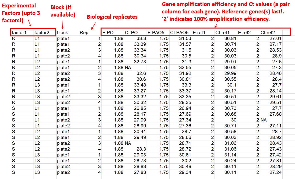
For relative expression analysis (using TTEST_DDCt, ANOVA_DCt, ANOVA_DDCt and REPEATED_DDCt functions), the amplification efficiency (E) and Ct or Cq values (the mean of technical replicates) is used for the input table. if the E values are not available you should use ‘2’ instead representing the complete primer amplification efficiency. The required column structure of the input data is:

Experimental condition columns (up to 3 factors, and one block if available)
Replicates information (biological replicates or subjects; see NOTE 1, and NOTE 2)
Target genes efficiency and Ct values (a pair column for each gene).
Reference genes efficiency and Ct values (a pair column for each gene)

The package supports one or more target or reference gene(s), supplied as efficiency–Ct column pairs. Reference gene columns must always appear last. A sample input data is presented below.

NOTE 1

For TTEST_DDCt, ANOVA_DCt, and ANOVA_DDCt, each row is from a separate and uniq biological replicate. For example, a dataframe with 12 rows has come from an experiment with 12 individuals. The REPEATED_DDCt function is intended for experiments with repeated observations (e.g. time-course data). For REPEATED_DDCt, the Replicate column contains identifiers for each individual (id or subject). For example, all rows with a 1 at Rep column correspond to a single individual, all rows with a 2 correspond to another individual, and so on, which have been sampled at specific time points.

NOTE 2

Your data table may also include technical replicates. In this case, the meanTech function should be applied first to calculate the mean of the technical replicates. The resulting table is then used as the input for expression analysis. To use the meanTech function correctly, the technical replicate column must appear immediately after the biological replicate column (see Mean of technical replicates for an example).

Data Analysis

Amplification Efficiency

The efficiency function calculates the amplification efficiency (E), slope, and R² statistics for genes, and performs pairwise comparisons of slopes. It takes a data frame in which the first column contains the dilution ratios, followed by the Ct value columns for each gene.

# Applying the efficiency function
data <- read.csv(system.file("extdata", "data_efficiency.csv", package = "rtpcr"))
data
dilutions   Gene1   Gene2   Gene3
1.00    25.58   24.25   22.61
1.00    25.54   24.13   22.68
1.00    25.50   24.04   22.63
0.50    26.71   25.56   23.67
0.50    26.73   25.43   23.65
0.50    26.87   26.01   23.70
0.20    28.17   27.37   25.11
0.20    28.07   26.94   25.12
0.20    28.11   27.14   25.11
0.10    29.20   28.05   26.17
0.10    29.49   28.89   26.15
0.10    29.07   28.32   26.15
0.05    30.17   29.50   27.12
0.05    30.14   29.93   27.14
0.05    30.12   29.71   27.16
0.02    31.35   30.69   28.52
0.02    31.35   30.54   28.57
0.02    31.35   30.04   28.53
0.01    32.55   31.12   29.49
0.01    32.45   31.29   29.48
0.01    32.28   31.15   29.26

# Analysis
efficiency(data)

$Efficiency
   Gene     Slope        R2        E
1 Gene1 -3.388094 0.9965504 1.973110
2 Gene2 -3.528125 0.9713914 1.920599
3 Gene3 -3.414551 0.9990278 1.962747

$Slope_compare
$contrasts
 contrast          estimate    SE df t.ratio p.value
 C2H2.26 - C2H2.01   0.1400 0.121 57   1.157  0.4837
 C2H2.26 - GAPDH     0.0265 0.121 57   0.219  0.9740
 C2H2.01 - GAPDH    -0.1136 0.121 57  -0.938  0.6186

Relative expression

Relative expression analysis can be done using $\Delta\Delta Ct$ or $\Delta Ct$ methods. Below is an example of expression analysis using $\Delta\Delta Ct$ method.

# An example of a properly arranged dataset from a repeated-measures experiment.
data <- read.csv(system.file("extdata", "data_repeated_measure_1.csv", package = "rtpcr"))
data

time    id  E_Target    Ct_target   E_Ref      Ct_Ref
   1     1      2       18.92   2   32.77
   1     2      2       15.82   2   32.45
   1     3      2       19.84   2   31.62
   2     1      2       19.46   2   33.03
   2     2      2       17.56   2   33.24
   2     3      2       19.74   2   32.08
   3     1      2       15.73   2   32.95
   3     2      2       17.21   2   33.64
   3     3      2       18.09   2   33.40

# Repeated measure analysis
res <- REPEATED_DDCt(
  data,
  numOfFactors = 1,
  numberOfrefGenes = 1,
  repeatedFactor = "time",
  calibratorLevel = "1",
  block = NULL)


# Anova analysis
ANOVA_DDCt(
  data,
  mainFactor.column = 1,
  numOfFactors = 1,
  numberOfrefGenes = 1,
  block = NULL)


# Paired t.test (equivalent to repeated measure analysis, but not always the same results, due to different calculation methods!)
TTEST_DDCt(
  data[1:6,], 
  numberOfrefGenes = 1, 
  paired = T)


# Anova analysis
data <- read.csv(system.file("extdata", "data_2factorBlock3ref.csv", package = "rtpcr"))
res <- ANOVA_DDCt(
  x = data,
  mainFactor.column = 1,
  numOfFactors = 2,
  numberOfrefGenes = 1,
  block = "block",
  analyseAllTarget = TRUE)

Output

Data output

A lot of outputs including relative expression table, lm models, residuals, raw data and ANOVA table for each gene can be accessed. The expression table of all genes is returned by res$combinedFoldChange. Other outpus for each gene can be obtained as follow:

Per_gene Output	Code
expression table	`res$combinedFoldChange`
ANOVA table	`res$perGene$gene_name$ANOVA_table`
ANOVA lm	`res$perGene$gene_name$lm_ANOVA`
ANCOVA lm	`res$perGene$gene_name$lm_ANCOVA`
Residuals	`resid(res$perGene$gene_name$lm_ANOVA)`

# Relative expression table for the specified column in the input data:
df <- res$combinedFoldChange
df
Relative Expression
gene   contrast       RE  log2FC pvalue sig    LCL     UCL     se Lower.se.RE Upper.se.RE Lower.se.log2FC Upper.se.log2FC
PO            R   1.0000  0.0000 1.0000     0.0000  0.0000 0.5506      0.6828      1.4647          0.0000          0.0000
PO       S vs R  11.6130  3.5377 0.0001 *** 4.4233 30.4888 0.2286      9.9115     13.6066          3.0193          4.1450
GAPDH         R   1.0000  0.0000 1.0000     0.0000  0.0000 0.4815      0.7162      1.3962          0.0000          0.0000
GAPDH    S vs R   6.6852  2.7410 0.0001 *** 3.0687 14.5641 0.3820      5.1301      8.7118          2.1034          3.5719
ref2          R   1.0000  0.0000 1.0000     0.0000  0.0000 0.6928      0.6186      1.6164          0.0000          0.0000
ref2     S vs R   0.9372 -0.0936 0.9005     0.3145  2.7929 0.2414      0.7927      1.1079         -0.1107         -0.0792

Plot output

A single function of plotFactor is used to produce barplots for one- to three-factor expression tables.

Plot output: example 1

data <- read.csv(system.file("extdata", "data_3factor.csv", package = "rtpcr"))
#Perform analysis first
res <- ANOVA_DCt(
  data,
  numOfFactors = 3,
  numberOfrefGenes = 1,
  block = NULL)
  
df <- res$combinedResults
 df
 # Generate three-factor bar plot
 p <- plotFactor(
  df,
  x_col = "SA",       
  y_col = "log2FC",       
  group_col = "Type",   
  facet_col = "Conc",    
  Lower.se_col = "Lower.se.log2FC",
  Upper.se_col = "Upper.se.log2FC",
  letters_col = "sig",
  letters_d = 0.3,
  col_width = 0.7, 
  dodge_width = 0.7,
  fill_colors = c("palegreen3", "skyblue"),
  color = "black",
  base_size = 14, 
  alpha = 1,
  legend_position = c(0.1, 0.2))

library(ggplot2)
p + theme(
  panel.border = element_rect(color = "black", linewidth = 0.5))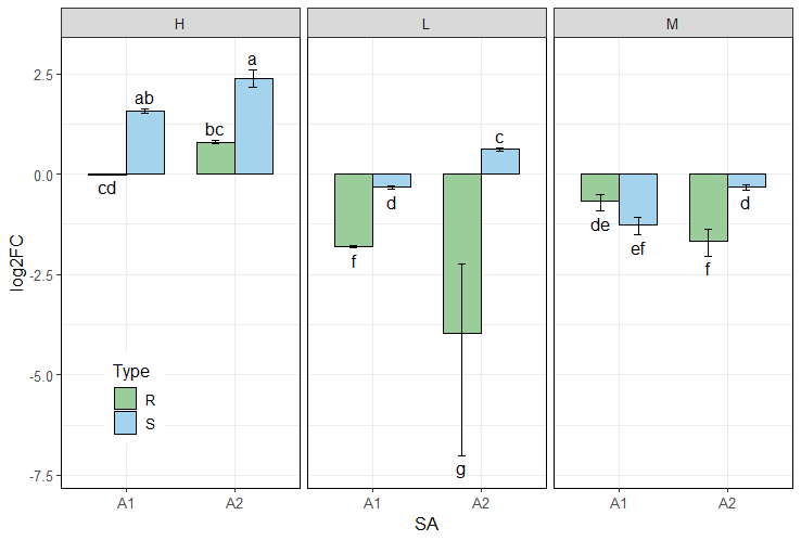

How to edit ouptput plots?

the rtpcr plotFactor function create ggplot objects for one to three factor table that can furtherbe edited by adding new layers:

Task	Example Code
Change y-axis label	`p + ylab("Relative expression ($\Delta\Delta Ct$ method)")`
Add a horizontal reference line	`p + geom_hline(yintercept = 0, linetype = "dashed")`
Change y-axis limits	`p + scale_y_continuous(expand = expansion(mult = c(0, 0.1)))`
Relabel x-axis	`p + scale_x_discrete(labels = c("A" = "Control", "B" = "Treatment"))`
Change fill colors	`p + scale_fill_brewer(palette = "Set2")`

Plot output: example 2

data <- read.csv(system.file("extdata", "data_2factorBlock.csv", package = "rtpcr"))
res <- ANOVA_DCt(data, 
      numOfFactors = 2,
      block = "block",
      numberOfrefGenes = 1)

df <- res$combinedResults

p1 <- plotFactor(
  data = df,
  x_col = "factor2",
  y_col = "RE",
  group_col = "factor1",
  Lower.se_col = "Lower.se.RE",
  Upper.se_col = "Upper.se.RE",
  letters_col = "sig",
  letters_d = 0.2,
  fill_colors = c("aquamarine4", "gold2"),
  color = "black",
  alpha = 1,
  col_width = 0.7,
  dodge_width = 0.7,
  base_size = 16, 
  legend_position = c(0.2, 0.8))

library(ggplot2)
p1 + 
  theme(axis.text.x = element_text(size = 14, color = "black", angle = 45),
        axis.text.y = element_text(size = 14,color = "black", angle = 0, hjust = 0.5)) +
  theme(legend.text = element_text(colour = "black", size = 14),
        legend.background = element_rect(fill = "transparent")) +
  scale_y_continuous(expand = expansion(mult = c(0, 0.1)))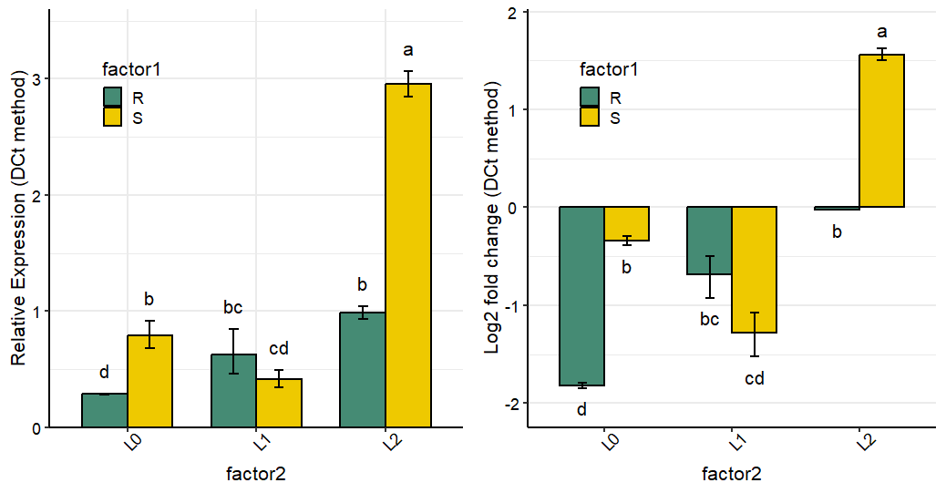

Plot output: example 3

# Heffer et al., 2020, PlosOne
library(dplyr)
df <- read.csv(system.file("extdata", "Heffer2020PlosOne.csv", package = "rtpcr"))

res <- ANOVA_DDCt(
  df,
  numOfFactors = 1,
  mainFactor.column = 1,
  numberOfrefGenes = 1,
  block = NULL)

data <- res$combinedFoldChange
data$gene <- factor(data$gene, levels = unique(data$gene))

# Selecting only the first words in 'contrast' column to be used as the x-axis labels.
data$contrast <- sub(" .*", "", data$contrast)

# Converting the 'contrast' column as factor and fix the current level order
data$contrast <- factor(data$contrast, levels = unique(data$contrast))

p <- plotFactor(
  data = data,
  x_col = "contrast",
  y_col = "RE",
  group_col = "contrast",
  facet_col = "gene",
  Lower.se_col = "Lower.se.RE",
  Upper.se_col = "Upper.se.RE",
  letters_col = "sig",
  letters_d = 0.2,
  alpha = 1,
  fill_colors = palette.colors(4, recycle = TRUE),
  color = "black",
  col_width = 0.5,
  dodge_width = 0.5,
  base_size = 16, 
  legend_position = "none")

library(ggplot2)
p + theme(
  panel.border = element_rect(color = "black", linewidth = 0.5)) +
  theme(axis.text.x = element_text(size = 14, color = "black", angle = 45, hjust = 1)) +
  xlab(NULL) +
  scale_y_continuous(expand = expansion(mult = c(0, 0.1))) +
  theme(
    strip.background = element_blank(),  # removes the faceting gray background
    strip.text = element_text(face = "bold")) # optional: keeps the text visible

Post-hoc analysis

The Means_DDCt function performs post-hoc comparisons using a fitted model object produced by ANOVA_DCt, ANOVA_DDCt or REPEATED_DDCt. It applies pairwise statistical comparisons of relative expression (RE) values for user-specified effects via the specs argument. Supported effects include simple effects, interactions, and slicing, provided the underlying model is an ANOVA. For ANCOVA models returned by this package, the Means_DDCt output is limited to simple effects only.

res <- ANOVA_DDCt(
  data_3factor,
  numOfFactors = 3,
  numberOfrefGenes = 1,
  mainFactor.column = 1,
  block = NULL)


# Relative expression values for Concentration main effect
Means_DDCt(res$perGene$E_PO$lm_ANOVA, specs = "Conc")

 contrast        RE        SE df       LCL       UCL p.value sig
 L vs H   0.1703610 0.2208988 24 0.1242014 0.2336757 <0.0001 ***
 M vs H   0.2227247 0.2208988 24 0.1623772 0.3055004 <0.0001 ***
 M vs L   1.3073692 0.2208988 24 0.9531359 1.7932535  0.0928 .  

Results are averaged over the levels of: Type, SA 
Confidence level used: 0.95 

# Relative expression values for Concentration sliced by Type
Means_DDCt(res$perGene$E_PO$lm_ANOVA, specs = "Conc | Type")

Type = R:
 contrast       RE        SE df       LCL      UCL p.value sig
 L vs H   0.103187 0.3123981 24 0.0659984 0.161331 <0.0001 ***
 M vs H   0.339151 0.3123981 24 0.2169210 0.530255 <0.0001 ***
 M vs L   3.286761 0.3123981 24 2.1022126 5.138776 <0.0001 ***

Type = S:
 contrast       RE        SE df       LCL      UCL p.value sig
 L vs H   0.281265 0.3123981 24 0.1798969 0.439751 <0.0001 ***
 M vs H   0.146266 0.3123981 24 0.0935518 0.228684 <0.0001 ***
 M vs L   0.520030 0.3123981 24 0.3326112 0.813055  0.0059 ** 

Results are averaged over the levels of: SA 
Confidence level used: 0.95 

# Relative expression values for Concentration sliced by Type and SA
Means_DDCt(res$perGene$E_PO$lm_ANOVA, specs = "Conc | Type * SA")

Checking normality of residuals

If the residuals from a t.test or an lm or and lmer object are not normally distributed, the significance results might be violated. In such cases, non-parametric tests can be used. For example, the Mann–Whitney test (also known as the Wilcoxon rank-sum test), implemented via wilcox.test(), is an alternative to t.test, and kruskal.test() is an alternative to one-way analysis of variance. These tests assess differences between population medians using independent samples. However, the t.test function (along with the TTEST_DDCt function described above) includes the var.equal argument. When set to FALSE, perform t.test under the unequal variances hypothesis. Residuals for lm (from ANOVA_DCt and ANOVA_DDCt functions) and lmer (from REPEATED_DDCt function) objects can be extracted and plotted as follow:

data <- read.csv(system.file("extdata", "data_repeated_measure_1.csv", package = "rtpcr"))
res3 <- REPEATED_DDCt(
  data,
  numOfFactors = 1,
  numberOfrefGenes = 1,
  repeatedFactor = "time",
  calibratorLevel = "1",
  block = NULL
)
residuals <- resid(res3$perGene$Target$lm)
shapiro.test(residuals) 
par(mfrow = c(1,2))
plot(residuals)
qqnorm(residuals)
qqline(residuals, col = "red")

Mean of technical replicates

Calculating the mean of technical replicates and generating an output table suitable for subsequent ANOVA analysis can be accomplished using the meanTech function. The input dataset must follow the column structure illustrated in the example data below. Columns used for grouping should be explicitly specified via the groups argument of the meanTech function.

# See example input data frame:
data <- read.csv(system.file("extdata", "data_withTechRep.csv", package = "rtpcr"))
data

# Calculating mean of technical replicates
meanTech(data, groups = 1:4)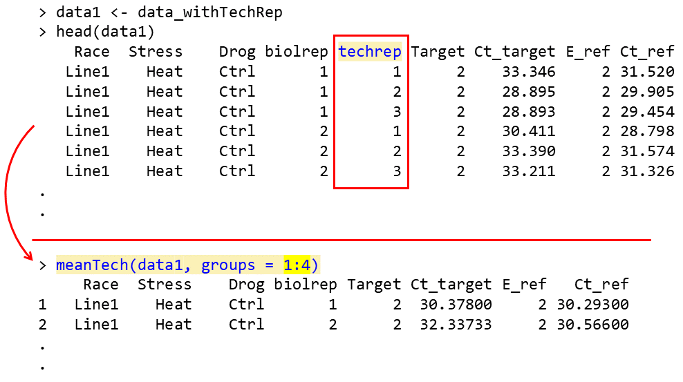

Contact

Email: gh.mirzaghaderi at uok.ac.ir

Citation

citation("rtpcr")

To cite the package ‘rtpcr’ in publications, please use:

  Ghader Mirzaghaderi (2025). rtpcr: a package for statistical analysis and graphical
  presentation of qPCR data in R. PeerJ 13:e20185. https://doi.org/10.7717/peerj.20185

A BibTeX entry for LaTeX users is

  @Article{,
    title = {rtpcr: A package for statistical analysis and graphical presentation of qPCR data in R},
    author = {Ghader Mirzaghaderi},
    journal = {PeerJ},
    volume = {13},
    pages = {e20185},
    year = {2025},
    doi = {10.7717/peerj.20185},
  }

Getting help

If you encounter a clear bug, please file a minimal reproducible example on github

References

Livak, Kenneth J, and Thomas D Schmittgen. 2001. Analysis of Relative Gene Expression Data Using Real-Time Quantitative PCR and the Double Delta CT Method. Methods 25 (4). doi.org/10.1006/meth.2001.1262.

Ganger, MT, Dietz GD, Ewing SJ. 2017. A common base method for analysis of qPCR data and the application of simple blocking in qPCR experiments. BMC bioinformatics 18, 1-11. doi.org/10.1186/s12859-017-1949-5.

Mirzaghaderi G. 2025. rtpcr: a package for statistical analysis and graphical presentation of qPCR data in R. PeerJ 13, e20185. doi.org/10.7717/peerj.20185.

Pfaffl MW, Horgan GW, Dempfle L. 2002. Relative expression software tool (REST©) for group-wise comparison and statistical analysis of relative expression results in real-time PCR. Nucleic acids research 30, e36-e36. doi.org/10.1093/nar/30.9.e36.

Taylor SC, Nadeau K, Abbasi M, Lachance C, Nguyen M, Fenrich, J. 2019. The ultimate qPCR experiment: producing publication quality, reproducible data the first time. Trends in Biotechnology, 37(7), 761-774. doi.org/10.1016/j.tibtech.2018.12.002.

Yuan, JS, Ann Reed, Feng Chen, and Neal Stewart. 2006. Statistical Analysis of Real-Time PCR Data. BMC Bioinformatics 7 (85). doi.org/10.1186/1471-2105-7-85.